Data Wrangling with R

Prerequsities

library(tidyverse) # today's package
library(gapminder) # data set

Recap

Common errors when reading file

not loading correct package
not attaching .csv extension
using wrong case
not using quotes "" around file name

Recap - `here` package

Type here() in your console. What do you see?

here()

[1] "/Users/meenakshikushwaha/Dropbox/R projects/github/data_wrangling_quarto"

Recap - `here` package

here tells R where your file is

If your data is in the main directory where here() begins

my_data <- read_csv(here("my_file.csv"))

If you are data is inside a folder

my_data <- read_csv(here("data", "my_file.csv"))`

If you are data is deep inside a subfolder

my_data <- read_csv(here("data", "sub_folder", "my_file.csv"))

Why not just use setwd()

Using here() makes your code more robust and shareable

Demo

What is `tidyverse`

A collection of R packages designed for data science. All packages share an underlying design philosophy, grammar, and data structures.

dplyr for data manipulation
ggplot2 for data visualizations
readr for reading data
stringr for string manipulation

Basics

Pick observations by their values filter()
Reorder the rows arrange()
Pick variables by their names select()
Create new variables with functions of existing variables mutate()
Collapse many values down to a single summary summarise(), used with group_by()

These six functions provide the verbs for a language of data manipulation

About the dataset

Gapminder dataset

Dataset of 142 countries, with values for life expectancy, GDP per capita, and population, every five years, from 1952 to 2007

country	continent	year	lifeExp	pop	gdpPercap
Afghanistan	Asia	1952	28.801	8425333	779.4453
Afghanistan	Asia	1957	30.332	9240934	820.8530
Afghanistan	Asia	1962	31.997	10267083	853.1007
Afghanistan	Asia	1967	34.020	11537966	836.1971
Afghanistan	Asia	1972	36.088	13079460	739.9811
Afghanistan	Asia	1977	38.438	14880372	786.1134

Gapminder dataset

head(gapminder, 15)

# A tibble: 15 × 6
   country     continent  year lifeExp      pop gdpPercap
   <fct>       <fct>     <int>   <dbl>    <int>     <dbl>
 1 Afghanistan Asia       1952    28.8  8425333      779.
 2 Afghanistan Asia       1957    30.3  9240934      821.
 3 Afghanistan Asia       1962    32.0 10267083      853.
 4 Afghanistan Asia       1967    34.0 11537966      836.
 5 Afghanistan Asia       1972    36.1 13079460      740.
 6 Afghanistan Asia       1977    38.4 14880372      786.
 7 Afghanistan Asia       1982    39.9 12881816      978.
 8 Afghanistan Asia       1987    40.8 13867957      852.
 9 Afghanistan Asia       1992    41.7 16317921      649.
10 Afghanistan Asia       1997    41.8 22227415      635.
11 Afghanistan Asia       2002    42.1 25268405      727.
12 Afghanistan Asia       2007    43.8 31889923      975.
13 Albania     Europe     1952    55.2  1282697     1601.
14 Albania     Europe     1957    59.3  1476505     1942.
15 Albania     Europe     1962    64.8  1728137     2313.

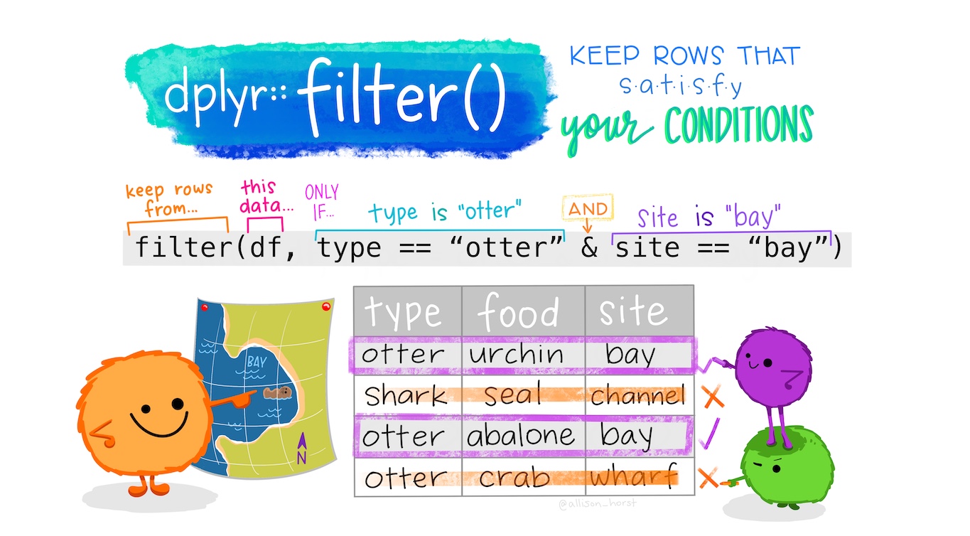
`filter()`

Keep or discard observations that satisfy certain condition

gapminder %>% 
  filter(country == "India")

country	continent	year	lifeExp	pop	gdpPercap
India	Asia	1952	37.373	3.72e+08	546.5657
India	Asia	1957	40.249	4.09e+08	590.0620
India	Asia	1962	43.605	4.54e+08	658.3472
India	Asia	1967	47.193	5.06e+08	700.7706
India	Asia	1972	50.651	5.67e+08	724.0325
India	Asia	1977	54.208	6.34e+08	813.3373

`filter()`

gapminder %>% 
  filter(country == "India", year < 1975)

country	continent	year	lifeExp	pop	gdpPercap
India	Asia	1952	37.373	3.72e+08	546.5657
India	Asia	1957	40.249	4.09e+08	590.0620
India	Asia	1962	43.605	4.54e+08	658.3472
India	Asia	1967	47.193	5.06e+08	700.7706
India	Asia	1972	50.651	5.67e+08	724.0325

Using the pipe `%>%`

simplifies your code
improves readability

filter(gapminder, country == "India")

is same as

gapminder %>% filter(country == "India")

Memory tip: %>% can be read as “and, then”

Keyboard shortcut Ctrl/Cmd + Shift + M

Quiz

How would you filter data from all asian countries that have life expectancy (lifeExp) higher than 80?

gapminder %>% filter(continent = “Asia”, lifeExp>“80”)
gapminder %>% filter(continent = “Asia”, lifeExp>80)
gapminder %>% filter(continent == Asia, lifeExp>80)

gapminder %>% filter(continent == “Asia”, lifeExp>80)

`filter()`

the | operator signifies “or”

gapminder %>% 
  filter(country=="India" | country == "Nepal")

country	continent	year	lifeExp	pop	gdpPercap
India	Asia	1952	37.373	372000000	546.5657
India	Asia	1957	40.249	409000000	590.0620
India	Asia	1962	43.605	454000000	658.3472
India	Asia	1967	47.193	506000000	700.7706
India	Asia	1972	50.651	567000000	724.0325
India	Asia	1977	54.208	634000000	813.3373
India	Asia	1982	56.596	708000000	855.7235
India	Asia	1987	58.553	788000000	976.5127
India	Asia	1992	60.223	872000000	1164.4068
India	Asia	1997	61.765	959000000	1458.8174
India	Asia	2002	62.879	1034172547	1746.7695
India	Asia	2007	64.698	1110396331	2452.2104
Nepal	Asia	1952	36.157	9182536	545.8657
Nepal	Asia	1957	37.686	9682338	597.9364

`filter()`

Using %in% to match more than one value

gapminder %>% 
  filter(year %in% c(1952,1962, 1972 ))

country	continent	year	lifeExp	pop	gdpPercap
Afghanistan	Asia	1952	28.801	8425333	779.4453
Afghanistan	Asia	1962	31.997	10267083	853.1007
Afghanistan	Asia	1972	36.088	13079460	739.9811
Albania	Europe	1952	55.230	1282697	1601.0561
Albania	Europe	1962	64.820	1728137	2312.8890
Albania	Europe	1972	67.690	2263554	3313.4222
Algeria	Africa	1952	43.077	9279525	2449.0082
Algeria	Africa	1962	48.303	11000948	2550.8169

`arrange()`

Arrange rows in asending order by default

gapminder %>% 
  filter(year %in% c(1952,1962, 1972 )) %>% 
  arrange(year)

country	continent	year	lifeExp	pop	gdpPercap
Afghanistan	Asia	1952	28.801	8425333	779.4453
Albania	Europe	1952	55.230	1282697	1601.0561
Algeria	Africa	1952	43.077	9279525	2449.0082
Angola	Africa	1952	30.015	4232095	3520.6103
Argentina	Americas	1952	62.485	17876956	5911.3151
Australia	Oceania	1952	69.120	8691212	10039.5956

`arrange()`

Arrange rows in descening order using desc

gapminder %>% 
  filter(year %in% c(1952,1962, 1972 )) %>% 
  arrange(desc(year))

country	continent	year	lifeExp	pop	gdpPercap
Afghanistan	Asia	1972	36.088	13079460	739.9811
Albania	Europe	1972	67.690	2263554	3313.4222
Algeria	Africa	1972	54.518	14760787	4182.6638
Angola	Africa	1972	37.928	5894858	5473.2880
Argentina	Americas	1972	67.065	24779799	9443.0385
Australia	Oceania	1972	71.930	13177000	16788.6295

Quiz

Select the code to arrange population (pop) in descening order

gapminder %>% filter(pop)

gapminder %>% arrange(desc(pop))

gapminder %>% arrange(pop)
gapminder %>% arrange(year)

`select()`

Select variables or columns of interest

gapminder %>% 
  select(country, year, pop)

country	year	pop
Afghanistan	1952	8425333
Afghanistan	1957	9240934
Afghanistan	1962	10267083
Afghanistan	1967	11537966
Afghanistan	1972	13079460
Afghanistan	1977	14880372

`select()`

Drop variables using -

gapminder %>% 
  select(-pop)

country	continent	year	lifeExp	gdpPercap
Afghanistan	Asia	1952	28.801	779.4453
Afghanistan	Asia	1957	30.332	820.8530
Afghanistan	Asia	1962	31.997	853.1007
Afghanistan	Asia	1967	34.020	836.1971
Afghanistan	Asia	1972	36.088	739.9811
Afghanistan	Asia	1977	38.438	786.1134

`select()`

There are a number of helper functions you can use within select():

starts_with(“abc”): matches names that begin with “abc”
ends_with(“xyz”): matches names that end with “xyz”
contains(“ijk”): matches names that contain “ijk”
matches(“(.)\1”): selects variables that match a regular expression
num_range(“x”, 1:3): matches x1, x2 and x3

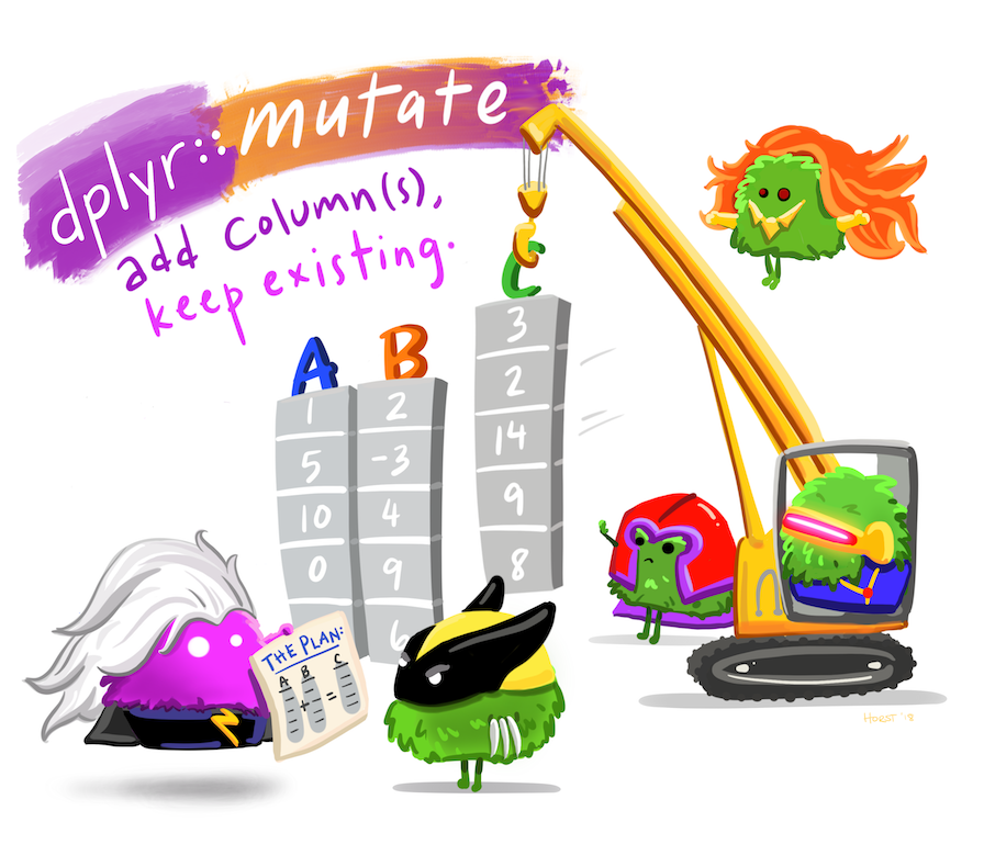
`mutate()`

Adds new variable at the end of your dataset

gapminder %>% 
  select(country, pop) %>% 
  mutate(pop_mil = round(pop/1000000, 1))

country	pop	pop_mil
Afghanistan	8425333	8.4
Afghanistan	9240934	9.2
Afghanistan	10267083	10.3
Afghanistan	11537966	11.5
Afghanistan	13079460	13.1
Afghanistan	14880372	14.9

`mutate()`

Some of the ways that you can create new variables

Arithmetic operators: +, -, *, /, ^
Modular arithmetic: %/% (integer division) and %% (remainder)
Logs: log(), log2(), log10(), etc.
Offsets: lead() and lag()
Logical comparisons: <, <=, >, >=, !=, and ==
Ranking eg. min_rank()

`mutate()`

Example

gapminder %>% 
  select(country, year, pop) %>% 
  mutate(pop_rank = min_rank(pop)) %>% 
  arrange(pop_rank)

country	year	pop	pop_rank
Sao Tome and Principe	1952	60011	1
Sao Tome and Principe	1957	61325	2
Djibouti	1952	63149	3
Sao Tome and Principe	1962	65345	4
Sao Tome and Principe	1967	70787	5
Djibouti	1957	71851	6

Quiz

What does the following code do?

gapminder %>% 
select(country, year, pop) %>% 
  mutate(pop_lakh = pop/100000)

Remove country, year and pop
Add new variables country, year , pop, and pop_lakh to the dataset

select country, year and pop from the dataset and add a new variable pop_lakh

All of the above

Using `mutate()` with a condition

Make a new variable with numeric code for each continent

gapminder %>% 
  select (country, continent, year, pop) %>% 
  mutate(cont_code = ifelse(continent == "Africa", 1, 
                            ifelse(continent == "Americas", 2,
                                   ifelse(continent == "Asia", 3,
                                          ifelse(continent == "Europe", 4, 5)))))

country	continent	year	pop	cont_code
Afghanistan	Asia	1952	8425333	3
Afghanistan	Asia	1957	9240934	3
Afghanistan	Asia	1962	10267083	3
Afghanistan	Asia	1967	11537966	3
Afghanistan	Asia	1972	13079460	3
Afghanistan	Asia	1977	14880372	3

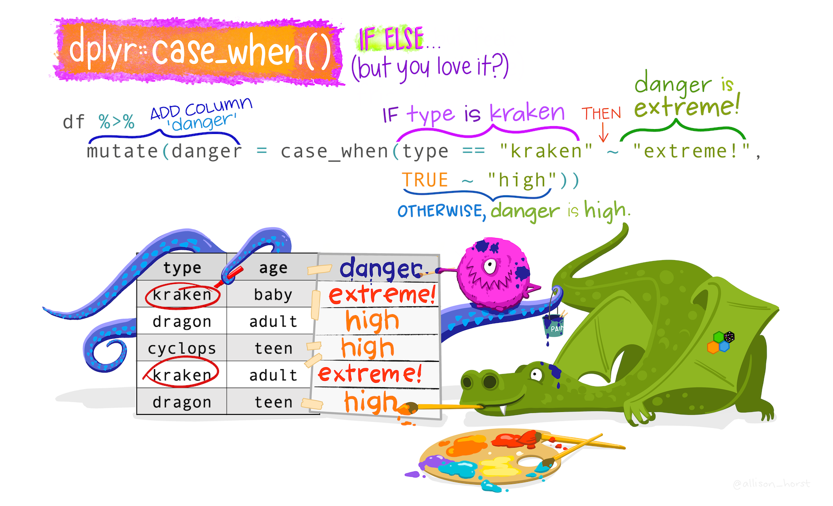
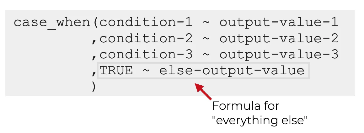
`case_when()`

Using `case_when()` with `mutate()`

gapminder %>% 
  select (country, continent, year, pop) %>% 
  mutate(cont_code = case_when(continent == "Africa" ~ 1,
                               continent == "Americas" ~ 2,
                               continent == "Asia" ~ 3,
                               continent == "Europe" ~ 4,
                               TRUE ~ 5))

country	continent	year	pop	cont_code
Afghanistan	Asia	1952	8425333	3
Afghanistan	Asia	1957	9240934	3
Afghanistan	Asia	1962	10267083	3
Afghanistan	Asia	1967	11537966	3
Afghanistan	Asia	1972	13079460	3
Afghanistan	Asia	1977	14880372	3

Using `case_when()` with `mutate()`

gapminder %>% 
  select (country, continent, year, pop) %>% 
  mutate(cont_code = case_when(continent == "Africa" ~ 1,
                               continent == "Americas" ~ 2,
                               continent == "Asia" ~ 3,
                               continent == "Europe" ~ 4,
                               TRUE ~ 5))

`summarise()`

collapse data frame to a single summary

gapminder %>% 
  summarise(mean_lifeExp = mean(lifeExp))

mean_lifeExp
59.47444

Often used with groupby() to summarise by groups

gapminder %>% 
  group_by(continent) %>% 
  summarise(mean_lifeExp = mean(lifeExp))

continent	mean_lifeExp
Africa	48.86533
Americas	64.65874
Asia	60.06490
Europe	71.90369
Oceania	74.32621

Useful summary functions

mean(), median()
sd(), IQR()
min(), max()
n()

Counts

Count number of observations in each group

gapminder %>% 
  count(continent)

continent	n
Africa	624
Americas	300
Asia	396
Europe	360
Oceania	24

gapminder %>% 
  group_by(continent) %>% 
  summarise(observations = n())

continent	observations
Africa	624
Americas	300
Asia	396
Europe	360
Oceania	24

Resources

R for Data Science Chapter 5
Slides made using Quarto
Art work by Allison Horst